Hebbian Logic Networks

The Emergence of Probabilistic Logic

from Formal Neural Networks

Ben Goertzel

Novamente LLC

November 17, 2003

The Hebbian Logic Network is a unique neural network architecture, in which the relationship between symbolic logic and neural net learning dynamic is fairly simple and clear. The architecture involves cell assemblies, Hebbian learning, and “neural maps” a la Gerald Edelman, but goes beyond these inspirations by suggesting particular internal structures and interconnection patterns between neural clusters. In this paper a conceptual description of the Hebbian Logic Network architecture is presented, and the most essential aspects are elaborated mathematically.

A key point is the relationship identified between probabilistic logic and Hebbian learning. Heuristic arguments and rough calculations are given, suggesting that a form of logical called probabilistic term logic (PTL), may spontaneously emerge from Hebbian Logic Networks.

Finally, an extension of the architecture called Variable-Enhanced Hebbian Logic Networks is proposed, which deals explicitly with quantified variables and related mechanisms from predicate logic.

1. Introduction

This paper gives a conceptual overview of a novel neural network architecture called the Hebbian Logic Network. The objective of this architecture is simple and ambitious: to bridge the symbolic-subsymbolic gap in cognitive science, by presenting a clear conceptual picture of how logic-like processes may emerge from neuron-like processes in a reasonably efficient and natural way.

The level of exposition is semi-technical. Complete and rigorous development of the Hebbian Logic framework will require extensive simulations and mathematical calculations, and will occupy much more than a single paper. The goal here is merely to get across the key conceptual ideas of the architecture; the many details will be explored in follow-up work.

The Hebbian Logic Network architecture is similar in spirit to Hebbian cell assemblies and Edelman’s neural-cluster-based “Neural Darwinist” networks, but it has many unique points not covered in any of these inspirations. It also has overlaps with two AI architectures, which are not neural net based, but share somewhat similar overall structures: Webmind (Goertzel et al, 2000) and, to a lesser extent, Novamente (Goertzel et al, 2002)

The most important technical insight underlying Hebbian Logic Networks is the notion of logic-friendliness – a formal concept that is used to argue that probabilistic reasoning (in a particular form called Probabilistic Term Logic, or PTL; Goertzel et al, 2003) can emerge from Hebbian Logic Networks equipped with appropriate parameter values. This particular emergence is what we call “Hebbian Logic.”

The basic Hebbian Logic Network architecture covers simple probabilistic inference but doesn’t extend to advanced logic involving variables and quantifiers. We present an extension called Variable-Enhanced Hebbian Logic Networks, that remedies this deficiency, but at the cost of introducing some extra complexity into the design. There may well be other ways to get phenomena analogous to variables and quantifiers into Hebbian Logic Networks.

Finally, a few comments on the relationship between Hebbian Logic Networks, neuroscience and AI may be appropriate.

Regarding neuroscience, we wish to emphasize that Hebbian Logic Networks are an abstraction and not intended as a detailed model of the human brain. Rather, they are intended to display, in a relatively simple form, general principles that are hypothesized to underly the cognitive operations of the human brain.

Regarding AI; we are not certain whether Hebbian Logic Networks would serve as an effective practical approach to artificial intelligence. The framework would need to be fleshed out significantly beyond what has been done here, in order to assess this. For our own currently practical AI work (the Novamente system; Goertzel et al, 2003), we are taking a less neurally-inspired approach. However, we do feel the Hebbian Logic Network approach has sufficient potential along these lines to merit further investigation.

2. Knowledge Representation using Cell Assemblies

In this section we outline a generalized formal neural network model, to be used in the analysis and discussions of the following sections. The model is somewhat more general than typical neural network models; for instance, it includes links that point to links as well as links that span nodes. Not all of this generality is needed for the simplest version of Hebbian Logic; but we will discuss aspects of Hebbian Logic that can make good use of it.

2.1 Formal Neural Networks

Define a formal neuron as an object that contains a real number called “activation.” Define a first-order formal synapse as an ordered pair of formal neurons, which contains a real number called “weight.” Next, define a k’th-order formal synapse as an ordered pair of entities (N,S), where N is a formal neuron and S is either a formal neuron or a formal synapse with order < k. A formal neural network, then, consists of a set of formal synapses, together with the neurons joined by the synapses, endowed with two functions that serve as dynamics: an update function and a learning function.

We will omit the adjective “formal” in most of the following discussion, referring to simply “neural networks,” “synapses” and “neurons”. When we discuss the actual biological entities corresponding to these terms, this will be made explicit.

Note that, in this formalization, we allow synapses that point to other synapses, as well as the standard synapses that point to neurons. Synapses must come from neurons, however. This is not a precise neurophysiological model, but nor is the standard assumption that synapses only point to neurons; for instance, the brain has dendrodendritic synapses that appear to act by modulating the passage of charge along other synapses (Cowan et al, 1999). The inclusion of synapses pointing to synapses is purposeful here; these will be used in the simple Hebbian learning rule below.

Mathematically, we may formulate this neural net model as follows:

N = space of formal neurons

I: N àZ, an indexing of the elements of N

S = space of formal synapses, each one of which is identified with a pair (x,y),

with x Î N and y ÎNÈS. The synapse identified with (x,y) will

generally be denoted xày. Each synapse has a finite order k as defined in

text earlier.

T = (discrete) space of time values, a subset of the real numbers R

Where A is any set, let S* = ÈS^k, k = 1,2,…

outgoing: N à S* ,

where outgoing(x) is the tuple of all formal synapses in S of the form xày,ordered according to the indices I(y)

incoming: N -> S*,

where outgoing(x) is the tuple of all formal synapses in S of the form yàx, ordered according to the indices I(y)

nbh: 2^N à N*,

where nbh(A) is the tuple of all formal neurons y so that

xày Îoutgoing(x) for some xÎA, ordered according to the indices I(y)

nbh^k: Nà N*,

defined by nbh^k(A) = nbh( nbh^k-1(A) )

a: N ´T à R, where a(x,t) is the activation of neuron x at time t

a^~: 2^N´T à R*, where a^~(Q,t), Q Í N, is a tuple containing the activations

of the formal neurons in Q at time t, ordered according to the

indexing I

w: S ´ T à R, where w(x,t) is the weight of synapse x at time t

w^~: 2^S´T à R*, where w^~(Q,t), Q Í S, is a tuple containing the weights

of the formal synapses in Q at time t, ordered according to the

indexing I

Where f: A ´ T à B is any function, define f^$: A ´ 2^T à B*, where

f^$(x,H), x ÎA , H Í T, is the set of values f(x,t) for tÎH, ordered

according to the ordering of T

hist: T à T* , where hist(t) = (t-s,…,t-1,t) for some fixed s

All standard neural net update and learning functions may be described schematically by:

a(x,t) = update( a^$(x,hist(t-1)), a^{~ $}(nbh(x),hist(t-1)), w^~$(incoming(x),hist(t-1)) )

w(xày ,t) = learn( w^$ (xày, hist(t-1)), a^$(x,hist(t-1)), a^$(y,hist(t-1)) )

Here, the latter equation only applies in the case of a first-order synapse; for higher-order synapses, the equation looks like

w(xày ,t) = learn( w^$ (xày, hist(t-1)), a^$(x,hist(t-1)))

since the target is a link and lacks an activation.

What these equations say is simple: The activation of a neuron at time t is given by the update function, which uses as input the recent activation of the neuron and other neurons in the neighborhood, and the weights of the synapses coming into the neuron. The weight of a synapse at time t is given by the learn function, which takes as input the recent history of the weight of the synapse and the recent history of the activations of the source and target neurons.

The exact nature of the update and learning functions that best model brain activity are not known; and the neural net literature is full of update and learning functions that are tuned for particular practical applications or computational experiments.

Here we will assume a standard update function, in which neurons have thresholds, and when the activation at a neuron passes the threshold, the neuron sends activation to other neurons, along its synapses. The amount of activation that goes from neuron A to neuron B is equal to a constant value (the “activation quantum”) multiplied by the weight of the synapse. Once a neuron has sent activation, its activation value decreases to zero. Activation also decays by a small amount over time.

The bulk of this paper is oriented toward defining a class of learning functions that are adequate to induce “emergent logical behavior” in a formal neural network. We will propose a learning function that is different from the standard form given above, and is of the form

learn( w^$ (xày, hist(t)), a^$(x,hist(t)), a^$(y,hist(t)) , stat(nbh^k(x), hist(t)) )

where stat is a “statistics” function summarizing some data about x’s general neighborhood. In general, stat may be thought of as a map into Rⁿ; in practice, here, stat will map into R. A learning rule involving such a stat function may be called “semi-local” rather than truly local.

2.2 Varieties of Cell Assembly Based Knowledge Representation

The next preliminary issue to address, before moving on to the main point of the paper, is: How can knowledge be represented in a formal neural network in a reasonably “natural” way?

To answer this question, we will first of all introduce the standard distinction between procedural and declarative knowledge. Declarative knowledge is knowledge of facts or suppositions – statements about some aspect of the world. Procedural knowledge is knowledge of how to do something.

Also, to talk about knowledge representation, we must introduce the notion of a subnetwork of a neural network. A subnetwork is a pair (A,B) Í (N,S) where B consists of precisely those synapses xày where x and y are both in A. In other words a subnetwork consists of a set of neurons and all the synapses linking between different neurons in this set.

Subnetworks lead to subnetwork activation states. A subnetwork activation state consists of the activation values of a subnetwork, at a given point in time. A subnetwork activation state is defined in terms of a vector zÎ Rⁿ, but must be formally considered as a function mapping (subnetwork, time point) pairs into “uncertain truth values” in [0,1]. If f_z is a subnetwork activation state corresponding to the vector z, and (A,B) is a subnetwork, then f( (A,B), t ) indicates the degree to which the neurons in A (ordered by the indexing I) have the activation values z at the given time t.

Next, a subnetwork weight state is similar to a subnetwork activation state, but refers to the weight values of the synapses in the subnetwork, at a given time. A subnetwork activation time pattern consists of a series of subnetwork activation states, corresponding to different times; and a subnetwork weight time pattern is defined analogously.

Note that subnetwork states and time patterns are not tied to particular subnetworks: they are predicates that apply to various subnetworks to various degrees.

These notions let us describe many ways that declarative knowledge may be stored in a formal neural network; for example:

· As a particular subnetwork

· As a subnetwork activation state

· As a subnetwork weight state

· As a pair (subnetwork weight state, subnetwork activation state), where the two subnetworks may or may not be identical

· As a subnetwork activation time pattern

· As a subnetwork weight time pattern

· As a pair (subnetwork activation time pattern, subnetwork weight time pattern), where the two subnetworks may or may not be identical

· As a pair (subnetwork weight state, subnetwork activation time pattern), where the two subnetworks may or may not be identical

· etc.

Intuitively speaking, all of these are ways of storing knowledge in “cell assemblies,” the latter being basically a term for subnetworks that have a much higher average link weight than the average subnetwork.

The difference between storing knowledge in particular subnetworks, and in subnetwork states or time patterns, is fairly significant. In the one case, a certain fixed cell assembly holds a piece of knowledge, and in the other case, a piece of knowledge is a pattern that may be repeated throughout the network, and may even be removed and then dynamically reconstituted.

For the remainder of this paper, we will make the specific assumption that a piece of declarative knowledge is stored in either

a subnetwork weight state, which is embodied in one or more actual subnetworks.
a pair (subnetwork weight state, subnetwork activation state), where the subnetwork involved in the weight state is a subset of the subnetwork involved in the activation state
a pair (subnetwork weight state, subnetwork activation time pattern), where the subnetwork involved in the weight state is a subset of the subnetwork involved in the activation time pattern

The subnetwork weight states involved in these representations are what we call “neural cluster classes” – these are classes of essentially-equivalent “neural clusters” or “subnetworks.” The subnetwork activation states or time patterns are what we call “neural maps” – they are related but not identical to Edelman’s neural maps. A neural map in our framework is a set of neural clusters that become active when a neural cluster in a particular class becomes active and “triggers” them. The combination of a trigger neural cluster with a distributed map of neural clusters, gives a combination of localized and globalized knowledge representation.

The various redundant subnetworks representing a given piece of knowledge may not be entirely identical, but are assumed to be very similar, hence representable to within a high accuracy by the same subnetwork weight state. This is basically the assumption that Hebb made in his original work on Hebbian learning: that knowledge is stored in the brain by patterns of synaptic conductance or (as it is called in formal neural net models) “weight.” The importance of repeated, slightly varied copies of the same subnetwork has been emphasized by Edelman (1988) among other neural theorists.

The reason for assuming here that knowledge is represented by subnetwork weight states (often with associated neural maps), is not that this is traditional, but rather that the emergence of uncertain logic from neural dynamics seems to work out cleanly this way, and significantly less so in the other representations considered. However, we consider it quite possible that, in future, mechanisms for the emergence of uncertain logic from other forms of declarative knowledge representation will be discovered.

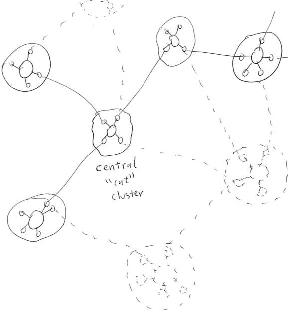
Figure 1

A “map” corresponding to the concept “cat”, consisting of a central “cat” cluster

whose activation triggers the activation of an attractor of interrelated neural clusters.

Next, procedural knowledge may also be stored in a neural network in more than one way. One way is to consider a procedure as a subnetwork of the form (A,B) where

A = Input È Hidden È Output

where the neurons in Input are considered as inputs and the neurons in Output are considered as outputs. Another way is to consider a procedure as a subnetwork weight time pattern, with the same tripartite interpretation of the subnetworks involved. These are both ways of storing procedural knowledge in “cell assemblies.” Again, we will consider a procedure as being embodied in a subnetwork weight state, instantiated by one or more particular subnetworks, and potentially associated with activation states or patterns in a broader subnetwork (consisting of a collection of neural clusters).

Discussion of more advanced general issues in knowledge representation will be deferred until Section 7. We now turn to some very specific issues regarding the representation of logical knowledge and the performance of inference on this knowledge via neural dynamics.

3. Representing Inheritance and Similarity in Neural Networks

In this section we specifically discuss the representation of two types of logical relationship that have foundational value in uncertain term logic: inheritance and similarity. We have discussed how to represent general relationships in neural network terms, using procedure-implementing subnetworks, subnetwork states or time patterns. But inheritance and similarity have a special role in uncertain logic, and will be treated separately. The essence of our linkage between neural net learning and symbolic logic lies in the way inheritance and similarity relationships between logical terms are proposed to emerge from linkages between neural net subassemblies.

3.1 Semantics of Inheritance and Similarity

Very roughly speaking, “A inherits from B” or Aà_I B, means that when B is present, A is also present. The truth value of the relationship measures the percentage of the times that B is present, that A is also present. “A is similar to B” or A «_S B, is a symmetrical version, whose truth value measures the percentage of the times that either one is present, that both are present.

A great deal of subtlety emerges when one examines the semantics of inheritance in detail (Goertzel et al, 2003). Many subtypes of the basic inheritance relation arise, dealing with such distinctions as intension vs. extension and group vs. individual. Here we will ignore these points and assume a simplistic approach to inheritance, considering Aà_I B to be basically interpretable as P(B|A). This is not incorrect, merely incomplete, since the more refined variations of inheritance may be interpreted as P(f(B)|f(A)) where the function f varies based on the inheritance type, or as weighted sums of several expressions of this nature..

3.2 Inheritance and Similarity as Emergent from Cell Assembly Linkage

In order to discuss the representation of logical relationships in neural networks, we will need to talk about links between subnetworks. These links exist on a different level from formal synapses, and are semantically quite different from them, which is why we have chosen to use different names for the connections at different levels (“links” versus “synapses”). Synapses actually exist in the data structures defining a formal neural network, and are intended to (somewhat loosely) represent physically existent entities in the brain. Links as we define them here are emergent entities, which represent patterns in a neural network, but are not explicitly embodied in the neural network’s data structures.

First we will associate with a subnetwork A and a time t a probability P(A,t), defined as the probability that, at time t, a randomly chosen neuron xÎA is firing.

The probability P(A)_t may then be defined as the average of P(A,s) over s in “recent history”. Often, in the following the time-dependence will be left implicit and we will write P(A)= P(A)_t. When the time-dependence is left implicit in an expression, the assumption is that all the probabilities in the expression refer averages over the same recent history, looking backwards from the same time t.

To discuss conditional probabilities, we must define an appropriate Boolean algebra on subnetworks. Where A and B are subnetworks, let AÈB denote the subnetwork consisting of all the neurons from A, all the neurons from B, and all synapses joining neurons from A or B to other neurons from A or B. Let AÇ B denote the subnetwork consisting of all neurons in both A and B, and all synapses whose source and target are both neurons in this set.

Then, where A and B are subnetworks, we may define the conditional probability P(A|B; t) = P(A ÇB,t)/ P(B,t), and a corresponding time-averaged variant

P(A|B)_t = å_r=0,…,N [w(r) P(A|B;t-r)]

where w(r) is monotone decreasing with å_r=0,… w(r) bounded. In the following, where A and B are subnetworks, we will generally use the shorthand P(A|B) to denote P(A|B)_t. This should not cause problems because the notion of a time-independent probability P(A|B) between subnetworks A and B does not exist.

If P(A|B) = p, we will write

Aà_I B

which is read “A inherits from B with strength p.”

We also define

A «_S B

to mean “A and B are similar”, or equationally s = P(AÇB | AÈB).

Note that

P(A ÇB| AÈB) = 1/ [1/P(A|B) + 1/P(B|A) – 1]

so that similarity values are actually implicit in inheritance values.

The network of inheritance and similarity links between subnetworks is a kind of “logical network” that exists on a higher level from the network of neurons and synapses, but is implicit in the latter, emergent from the latter, and evolves implicitly based on the dynamics of the latter. When we say that a link such as Aà_IB “exists in” a neural network, what we mean is that it emerges from the network according to the above definition, not that it is explicitly represented in the network by a synapse or any other particular structure.

3.3 Direct Embodiment

Finally, we introduce the important notion of a directly embodied relationship. Where A and B are two subnetworks in a neural network, we say that the relation Aà_I B is directly embodied if it would hold in a neural network consisting only of A B, and subjected to random stimulation. The random stimulation should be assumed to work as follows: each neuron in A is stimulated at time t with probability P(A); each neuron in B is stimulated at time t with probability P(B). The idea is that, if Aà_I B is directly embodied, then the relationship is embodied in the links between A and B, rather than implicitly in the links outside of the two subnetworks.

We may consider direct embodiment as a fuzzy relationship, in which case the degree of direct embodiment of R=”Aà_I B ” is the maximum similarity between R and any relationship present in the neural net A B under random stimulation as described above.

This definition requires us to define the similarity between two propositions (such as Aà_I B and Aà_I B <r>, or Aà_I B and Aà_I C , etc.)? This is easy to define if one has a framework for higher-order inference, as discussed in (Goertzel et al, 2003; Wang, 1995), and as briefly reviewed in the following section. The similarity between two relations R and S may simply be defined as the strength of the higher-order similarity relationship R «_S S. Basically, in a PTL context this indicates

P(R and S are both true | either R or S is true)

If Aà_I B exists in the network but is not directly embodied, we will say that it is indirectly embodied. It is possible for Aà_IB <p₁> to exist in the network as a whole, but Aà_IB<p₂> to be the strength of the inheritance from A to B in a randomly stimulated network consisting only of A and B, where s₁ and s₂ are very different.. In this case, there is no significantly directly embodied relationship involved.

4. Uncertain Term Logic

This section gives a quick overview of a general form of logic called uncertain logic (UTL), and then presents a specific variant of UTL called probabilistic term logic (PTL). This is preliminary work for the following section, where it is shown how neural net dynamics can be made to give rise to an approximate version of the actual inference rules of PTL. A full description of PTL is not possible within the scope of this paper; many details will be omitted, but the crucial formulas will be presented.

Term logic traces back to Aristotelian and Charles S. Peirce; it differs from the more standard predicate logic in a couple ways:

In their formal language, for simple statements term logic requires the subject-predicate form (SàP, some kind of inheritance), where both terms are from the same term space; predicate logic requires the predicate-argument form (P(x,y,z)), where predicates and arguments belong to two separate spaces.
The basic inference rule in term logic is (various forms of) syllogism, where the premises are SàM and MàP, and the conclusion is SàP; the basic inference in predicate logic is modus tollens, where M and MàP yield P.

The basic term logic inference rules are given diagrammatically in Figure 2, where each arrow indicates an inheritance relationship, the dotted arrows indicating premises and the solid arrows indicating conclusions.

Figure 2

Rules of Uncertain Term Logic

Crisp term logic deals only with propositions that are definitely true or definitely false; uncertain term logic deals with propositions that have non-boolean truth value. In the simplest case, uncertain term logic deals with truth values in the interval [0,1]. In some cases it’s also interesting to consider multidimensional truth value, for instance truth value that consists of a multiparameter probability distribution, or truth value consisting of a (strength, confidence) or (strength, confidence, weight of evidence[1]) tuple. Here however we will deal only with the simplest case, a truth value tv that equals a single value in [0,1], which we’ll call strength and which is interpretable as a conditional probability.

	Deduction	Abduction	Induction	Revision
1st premise	B à_I C <tv₁>	C à_I A <tv₁>	A à_I C <tv₁>	A à_I B <tv₁>
2nd premise	Aà_I B <tv₂>	B à_I A <tv₂>	A à_I B <tv₂>	A à_I B <tv₂>
conclusion	A à_I C <tv>	B à_I C <tv>	B à_I C <tv>	Aà_I B <tv>

There is more than one kind of uncertain term logic, including the NARS system due to Pei Wang (1995), and the PTL (Probabilistic Term Logic) system described in (Goertzel et al, 2003), which is similar to NARS in many regards but uses different truth value functions when managing uncertain evidence. For the purposes of this paper we will stick with PTL, because this is the system that, at this stage, appears to most vividly reveal the parallels between logic and neural nets.

The revision rule is essentially a weighted averaging rule. In Hebbian Logic Networks, this is taken care of by explicitly, by an “averaging subcluster” that lives at the center of a neural cluster. The other inference rules are subtler, and are viewed as emerging implicitly from Hebbian learning with appropriate parameter values – a longer story that will be unveiled in Section 6 below.

There are also term logic rules for dealing with similarity links; these follow directly from the corresponding rules for inheritance links, and will not be explicitly presented here.

4.1 Basic PTL Inference

In PTL, the deduction, induction and abduction rules emerge directly from elementary probabilistic considerations. This section gives an overview of the principles from which the rules are derived, and then a statement of the rules themselves. Derivation of the rules is given in (Goertzel et al, 2003); the treatment here is a brief summary of the relevant calculations.

In the case of each inference rule, one assumes one is given three sets of entities A, B, and C, and knowledge of the strengths of two inheritance relationships among these sets. One then wishes to derive the strength of the third inheritance relationship.

This reduces to the problem: given |AÇB| and |B ÇC|, estimate |AÇC|. As is apparent from observing the relevant Venn diagram

there is no necessary relationship here. But if one assumes that all unknown evidence is randomly distributed, one can make a statistical estimate. I.e., if we assume we know nothing about |A Ç C| a priori, then we can assume its properties are due to the random co-memberships of A and C. The problem of estimating |A Ç C| is then reducible to two standard combinatorics problems of selecting balls from a bag: one regarding |A Ç C Ç B| (here the bag is B) and the other regarding |A Ç C Ç ~B| (here the bag is ~B).

After doing the algebra, one obtains the following formula

|AÇ C| = |A ÇB|*|BÇ C|/|B| + (|A}-|AÇB|)(|C|-|BÇC|)/(|U|-|B|)

where U is the implicit universal set. This yields the deduction rule

Aà_IB <p₁>

B à_I C <p₂>

----------

Aà_I C

where

p = p₁ p₂ + (1-p₁)(P(C) – p(B)p₂)/(1-p(B))

Induction and abduction rules can be derived from this one. In the induction case, for example, we know the strength of B à_I A and B à_I C, and desire to compute the strength of A à_I C. But we can estimate the strength of Bà_I A from the strength of Aà_I B, via the “Bayes’ rule” formula P(B|A) = P(A|B) P(B)/P(A), and thus derive an induction formula from the above deduction formula.

Similarly, in the abduction case, we know Aà_I B and Cà_I B, and we desire Aà_I C; but we can estimate Cà_I B from Bà_I C using P(C|B) = P(B|C) P(C)/P(B).

Finally, Bayes’ rule can also be turned around to yield a “node probability” inference formula, which estimates P(A) given P(B), P(B|A) and P(A|B).

These simple formulas deal only with the “strengths” (probabilities) associated with inheritance relationships; they but they can be extended to deal with more distributional information.

4.2 Relational and Higher-Order Inference

Extending this approach to deal with relational inference is not difficult, if one introduces a “list” (tuple) operator as a primitive. While that is the approach we will take here, we note that lists are not the only option. For example, one alternative is to use higher-order functions and currying, as in combinatory logic (Curry and Feys, 1958). Of the options we’re aware of, however, lists seem the most natural in a neural network context.

Consider as an example the ternary relation (A,B,C). This can be represented as the inheritance relation

(A,B,C) è R

Inference can be done using these inheritance relationships, assuming one introduces elementary operators for accessing elements of lists.

The neural expression of lists is not difficult. Above we introduced the idea of a multipart Input space, Input = Input₁ È… È Input_{n .} This is a list, and it may be made more “listlike” by assuming that the different parts of the space Input_i are tightly-intralinked subnetworks.

Higher-order inference can also be easily incorporated into UTL, if one allows relations to join other relations. For instance, the relation “Pei believes the Earth is flat” can be represented as

(Pei, Earth è_Iflat) à_I believes

There is no conceptual problem with defining the conditional probability P(A|B) where A or B are relationships; one must merely consider P(B), for example, as the probability that the relationship B holds.

Neurally, if relationships are implemented as subnetwork states or temporal patterns, then higher-order relationships are simply other subnetwork states or temporal patterns, having their argument subnetwork states or temporal patterns as components.

4.3 Boolean Operators

What about Boolean combinations of terms or relationships? The simplest approach is to assume that AND, OR and NOT are explicitly represented as procedures. This is not a problem from the neural network perspective; the implementation of these logical operators as small neural subnetworks is well known.

In PTL and NARS alike, one assumes default truth value rules for AND, OR and NOT, namely

A <p₁>

B <p₂>

A AND B

p = p₁ * p₂

A <p₁>

B <p₂>

A OR B

p = p₁ + p₂ - p₁ * p₂

A <p₁>

NOT A

p = p₁

In PTL, these rules are applied only when the system has no specific “interdependency” information regarding the terms combined using the logical operators.

4.4 Variables, Quantifiers and Combinators

Perhaps the subtlest part of logic is the handling of variables and quantifiers. These are needed not only for advanced mathematics, but also for the representation and manipulation of certain relationships described in everyday language. The handling of variables and quantifiers (or their equivalents) in a neural net context is a subtle issue, which we have not yet fully resolved; but we will present some hypothetical ideas in this direction in Section 7 below.

To highlight the issues involved, consider for instance the difference between

1) Boys love dogs

2) Every boy has a dog he loves

To fully capture the sense of the latter, one needs to create something semantically equivalent to:

ForAll boys B, ThereExists dog D so that (loves, B,D)

If one is willing to explicitly admit existential quantifiers, and quantifier binding (the quantifier on D is bound to the quantifier on B, via a relation that logicians call a “Skolem function”), then this sort of situation can be dealt with consistently with uncertain term logic. In Section 7 below, we will describe an approach to expressing variables and quantifiers in a Hebbian Logic Network framework.

An alternate strategy is to avoid explicit use of quantifiers and variables, by using combinators (special higher-order relationships acting on relationships; Curry and Feys, 1958) instead. Combinatory logic allows the representation of complex quantified formulas without variables. With the combinator approach, one represents complex quantified expressions using procedures. But we know how to implement procedures in a formal neural network; this was discussed above. The basic combinators {S,K,B,C,I} used in combinatory logic have neural-net implementations. This is an approach that interests us, as we use combinatory logic heavily in our Novamente AI system. However, we have not yet discovered any neural-net implementation of combinatory logic or any variant thereof which is simple enough to be worth discussing in detail.

5. Hebbian Learning

In this section we discuss Hebbian learning, in preparation for our later treatment of the emergence of probabilistic inference from Hebbian learning in Hebbian Logic Networks. The “Hebbian” neural net learning rules proposed here for use in Hebbian Logic Networks are a little different form the standard variants of Hebbian learning; but, as we shall see, they follow the same basic conception.

There is no current evidence that the brain uses the Hebbian learning variants presented here; however, there is much evidence that the brain’s implementation of synaptic modification is very complex, significantly more so than any simplified “neurons as nodes and synapses as links” formal neural network model can capture (see e.g. Bi and Poo, 1999; Tao et al, 2000). Our hypothesis as regards neurophysiology is not that the human brain exactly follows the Hebbian logic rules given here, but rather that the brain, with its more complex neurons and its diversity of neurotransmitters, does something similar in effect to the Hebbian logic rules.

In fact, the specific rules given here are presented largely as illustrative examples. More critical is the general concept of a logic-friendly learning rule. Any learning rule fulfilling the general “logic-friendliness” criterion given below is, we will argue, capable of giving rise to PTL-style logical inference – implicitly and automatically. The simple Hebbian learning rules given below are – we propose -- examples of logic-friendly learning rules, the human brain may manifest other examples, and clever neural net designers may well conceive yet others.

5.1 Traditional Hebbian Learning

The original Hebbian learning rule, proposed by Donald Hebb in his 1949 book, was roughly

The weight of the synapse xày increases (by amount a₁) if x and y fire at roughly the same time
The weight of the synapse xày decreases (by amount a₂) if x fires at a certain time but y does not

Here I’ll call this Hebbian learning variant A. The dependency of a₁ and a₂ on various factors has been defined in different ways by different theorists.

Over the years since Hebb’s original proposal, many neurobiologists have sought evidence that the brain actually uses such a method. What they have found, so far, is a lot of evidence for the following learning rule (which I’ll call variant B):

The weight of the synapse xày increases if x fires shortly before y does
The weight of the synapse xày decreases if x fires shortly after y does

The new thing here, not foreseen by Donald Hebb, is the “postsynaptic depression” involved in rule component 2.

Of course, this rule does not sum up all the research recently done on Hebbian -type learning mechanisms in the brain. The real biological story underlying these approximate rules is quite complex, involving many particulars to do with neurotransmitters. Ill-understood details aside, however, there is an increasing body of evidence that not only does this sort of learning occur in the brain, but it leads to distributed experience-based neural modification: that is, one instance synaptic modification causes another instance of synaptic modification, which causes another, and so forth (Bi et al, 1999). This has been observed in “model systems” consisting of neurons extracted from a brain and hooked together in a laboratory setting and monitored.

5.2 Extending Hebbian Learning to Subnetworks

These rules are conventionally formulated in terms of individual neurons, but, they extend immediately to subnetworks. Define a synaptic pathway of length k as a series S of synapses S₁,…,S_k, so that for k+1 neurons, N₀,…,N_k, we have

S_r = N_r-1à N_r

If N₀ ÎA and N_k ÎB, then we say that S is a synaptic pathway from A to B. In this context, the neurons along the pathway S that are not in either A or B are called the intermediate neurons of the pathway S.

The “weight” of a pathway from A to B may be defined by the following experiment. Let r denote the number of intermediate neurons in the pathway. Fix a time interval T equal to c*r time steps, where a single time step is the time it takes charge to travel along a synapse from one neuron to another, in the formal neural network model. Then, take a network that is entirely quiescent except for the neurons in A, and let:

X = the amount of charge coming into the pathway from A at a time point t

Y = the amount of charge that comes out of the pathway into B at time t+T.

The ratio Y/X is an estimate of the weight of the synaptic pathway. Average this ratio over a large number of experiments, and you have a definition of the weight of the pathway from A to B.

In a similar way, one may define the weight of a bundle of (possibly overlapping) pathways from A to B. Given two subnetworks A and B, define the k-step synaptic linkage of A and B as the weight of the bundle of all synaptic pathways from A to B, with length k or less.

The Hebbian rule variants mentioned above carry over naturally to subnetworks and synaptic linkages. For instance, in either Hebb rule variant, if one has two subnetworks A and B, and a lot of neurons in A fire at time t, whereas a lot of neurons in B fire at time t+T, then overall the weights of a lot of synapses pointing from A to B will be increased, resulting in an increase in the r-step synaptic linkage between A and B.

Hebb learning variant A, for example, results in the following rules on the subnetwork level:

1. The weight of the synaptic linkage Aà_S B between A and B increases if A is active shortly before B is

2. The weight of the synaptic linkage Aà_S B decreases if A fires when B doesn’t

Hebb rule Variant B may be similarly formulated on the subnetwork level.

5.3 Logic-Friendly Learning Rules and PTL Compliance

Now we are prepared to begin moving toward the main point of the paper. On the one hand, we have PTL reasoning rules, and on the other hand, Hebbian learning. We have seen how the basic data structures used by PTL -- inheritance and similarity links -- can be understood to emerge from a neural network, as probabilistic relations between cell assemblies. But do Hebbian learning dynamics give rise to PTL inference rules on the emergent level? It seems that the standard variants of Hebbian learning do not. But, if one applies the right conceptual framework, one can find closely related, albeit more complex semi-Hebbian learning dynamics that do.

The approach I take here to finding such learning dynamics is “top-down” in nature. I ask: What principle need a learning rule obey in order to give rise to PTL? I enounce such a principle, and then I propose a relatively simple example of a learning rule that appears to obey this principle, to within a reasonable degree of approximation.

The basic conceptual framework proposed here is given by the following semi-rigorous definitions and hypothesis:

Definition 1:

A neural net learning rule R is logic-friendly if it has the following property: If P(A) P(B) is reasonably large, and AàB , then learning according to rule R will, with a high probability, modify the synaptic weights so that A à B is a directly embodied relationship in the neural net.

Definition 2:

Define the basic logical model L(N,t) of a neural network N at a given time t, as the set of all directly embodied inheritance and similarity relationships between subnetworks of N.

Definition 3:

A neural network is PTL-compliant to the extent that the relationships in L(N,t+1) follow from the relationships in L(N,t) according to the rules of PTL. To calculate the extent, take each relationship R in L(N+1,t), and calculate the minimum distance from R to any Q that follows from L(N,t) according to the rules of PTL. Then average these distances over all relationships in L(N+1,t).

Hypothesis 1:

A neural net equipped with a logic-friendly learning rule will be strongly PTL-compliant

Obviously, this is not a fully rigorous proposition because it is not quantified. For sake of simplicity, the definition of logic-friendliness above was left semi-formal. A rigorous formulation would have to estimate the strength of the PTL compliance in terms of the degree of logic-friendliness and other aspects of the learning rule and neural network. This is a valuable pursuit, but one that would drastically complicate the discussion, and we will not pursue this direction here.

In the following subsections we will give examples of simple Hebbian-like learning rules that appear to be logic-friendly.

We now give a proof-sketch of Hypothesis 1, semi-formally in the spirit of the semi-formal Hypothesis statement.

Consider for example the case of deduction. Suppose we have

AàB <p₁>

BàC <p₂>

as directly embodied relationships in the network Then it will empirically be true, generally speaking, that

AàC

where s is close to the number predicted by PTL. And the definition of a logic-friendly learning rule means that, if such a learning rule is in place, then if s is sufficiently large or sufficiently small, AàC will become directly embodied with a high probability.

The exact PTL formula follows if one makes appropriate independence assumptions. These will not always be exactly satisfied, but they will often be closely satisfied.

The same sort of argument holds for inductive and abductive reasoning. We see that emergent PTL is not precisely achieved by putting in place a logic-friendly learning rule, but it is approximately implemented. The deviations of logic-friendly learning from PTL are going to be significant, due to multiple causes, chiefly noise and the violation of independence assumptions. But, deviations from independence may be handled via procedures and higher-order inference, as is done in Novamente. And, a neural network need not do perfectly accurate probabilistic reasoning in order to give rise to significant intelligence. Indeed, it is well known that in most contexts humans are not accurate with the quantitative aspects of probabilistic inference (Wang, 1995).

6. Probabilistic Logical Inference Achieved through Neural Network Dynamics

Now we get to the crux of the Hebbian Logic approach. We have seen how logical knowledge can be represented in neural network terms, but the possibility of this representation is not really news: it was implicit in McCullough and Pitts’ foundational paper on neural networks, when they showed that a simple formal neural network can serve as a Universal Turing Machine. Anything finitely describable can be represented in a neural network, if one tries hard enough. The trick is to represent logical knowledge in a neural network in such a way that logical reasoning comes naturally out of the neural net dynamics. This section explains how the combination of probabilistic term logic with cell-assembly-based knowledge representation can pull this trick off, if one makes the right assumptions about the underlying neural net learning rule. The concepts of logic-friendliness and PTL-compliance introduced above will serve as a partial guide.

There are two main ideas presented in this section:

An architecture for the interior of neural clusters, which causes neural clusters to implement the revision rule
A variant of Hebbian learning which is semi-local rather than local, and which causes the dynamics of weight modification between neural clusters to embody conditional probabilities (hence causing the system to behave “as if” it were doing PTL deduction and inversion, i.e. achieving PTL-compliance)

6.1 The Internal Structure of Hebbian Logic Clusters

In order to achieve an analogue of the PTL revision rule, we propose that neural clusters representing declarative knowledge should have a special structure, consisting of:

a “central core” subcluster, which averages the inputs it receives from the peripheral subclusters
a set of peripheral subclusters, each of which exists to connect with some other particular cluster (and which adds together, rather than averaging, the activation along the links arriving from that other cluster)

In the simplest case, each peripheral subcluster represents a pair of inheritance relationships between the cluster A and some other particular cluster B (the relationships AàB and BàA). The central core effectively performs the PTL revision rule (which is a form of weighted averaging), revising the results produced by the peripheral subclusters. The use of this sort of revision will become clear a little later when we discuss the emergence of PTL deduction from Hebbian learning between clusters.

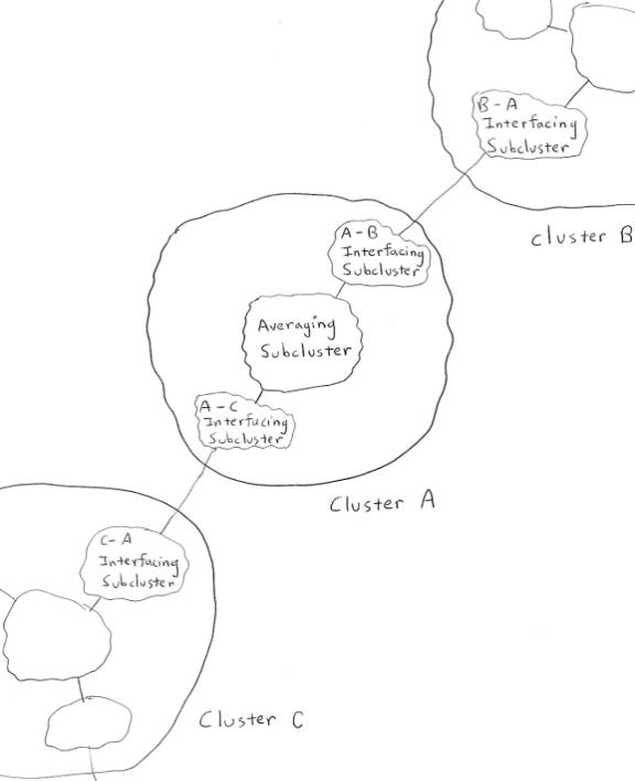
Figure 3

The internal structure of a Hebbian Logic Network cluster: an averaging subcluster that averages the outputs of the interfacing subclusters that surround it (each of which sums up the inputs from some other particular cluster)

6.2 Example Hebbian Logic Rules

Now it’s time to give a concrete example of a logic-friendly learning rule. In this subsection we will do some rough, heuristic arithmetic involving Hebbian learning variant A. Our aim is to show that, if the parameters are set right, then this sort of Hebbian learning, embedded in a Hebbian Logic Network architecture, can give rise to PTL inference.

Let us assume that we have a neural network containing an indirectly embodied relationship Aà_IC , where P(A) P(C) is fairly large (significantly larger than would be expected for two randomly chosen subnetworks). Then it will happen that when A is active, C becomes active fairly shortly afterwards, and both variants of Hebbian learning given above will then build links between neurons in A and neurons in C. This will create a directly embodied relationship Aà_I C <p₁>. The question is, what will be the strength p₁of this new directly embodied relationship? This depends on the parameters of the processes involved, which must be properly set in order for the emergence of accurate probabilistic logical inference to occur.

One act of synaptic-strength augmentation will occur each time that a neural firing in A is shortly followed by a neural firing in C. So, each time a neuron in A fires, the probability of an act of synaptic-strength augmentation occurring on some synapse joining A to C is equal to the strength p=P(C|A)_t of the relation Aà_I C . It follows that the expected amount of strength augmentation of synapses between A and C, over a period of time of duration D, is roughly equal to

S = D * P(A) * a₁ * p.

Of course, this kind of learning will lead to synapses becoming maximally strong when the duration D gets long enough, so we must assume a “decay” factor counteracting the ongoing synaptic weight enhancement. For simplicity of analysis, let’s assume that synaptic weights decay in magnitude by a constant factor d, and are incremented by Hebbian learning as described above. We then have a formula

S(t+1) = d*S(t) + P(A) * a₁ * p

and if we assume stationarity over a period of time, this converges to a fixed point

S = (P(A) * a₁ * p )/(1-d)

(Approximate stationarity will lead to approximate convergence; this is a well-behaved sort of iteration.)

Next, we may express the directly embedded probability AàC <p₁> roughly as

p₁ = q * S

What this says is that the chance that an activation in A is followed by an activation in C increases roughly proportionally to the total synaptic linkage between A and C.

In order to achieve p₁=p, which is what the definition of logic-friendliness requires, we must have

1 = q * P(A)*a₁/(1-d)

which can be achieved by setting

a₁ = (1-d)/ [q * P(A) ]

The annoying thing about this formula is the occurrence of P(A), which is not constant. This means that the increment in the Hebbian learning rule applied to synapse xày must depend (inversely) upon the amount of activity in the subnetwork to which the source belongs. This is not a local quantity, meaning that we do not have a fully local learning rule.

However, although the rule thus derived is not local, it is semi-local, in the sense that the parameters of a synapse’s learning rule rely only on the cell assemblies to which the source and target of the synapse belong. If one assumes – as is done in the Hebbian Logic Network architecture -- that the knowledge-representing cell assemblies in the neural network are disjoint, i.e. forming relatively well-distinguished clusters, then there is no tremendous problem with having cell-assembly-dependent parameters. It would be nice to get rid of this semi-locality and have a purely local approach, but there seems no ready way to do so. It is possible that it is precisely the need for this sort of semi-locality that has led all variants of Hebbian learning hitherto explored to behave so disappointingly.

Finally, we assumed in the above discussion that we were dealing with “an indirectly embodied relationship Aà_IC , where p is fairly large, significantly larger than would be expected by chance.” What if, on the other hand, we have an indirectly embodied relationship Aà_IC , where p is small, significantly smaller than would be expected by chance? This means that A and C are strongly anticorrelated, to use standard neural net language. In this case, part 2 of Hebbian learning variant A says that the synapses from A to C will have their weights decremented. This leads to an equation

S(t+1) = d*S(t) - P(A) * a₂ * p

(identical to the one above but with a different sign) and to a decrement formula

a₂ = - a₁

Thus we see that, in a probabilistic reasoning context, part 1 of Hebbian learning variant A takes care of positive evidence, whereas part 2 of Hebbian learning variant A takes care of negative evidence.

6.2.1 The Role of Averaging Subclusters

The role of the “averaging subclusters” in the Hebbian Logic Network architecture is an interesting one, which we will here explore by means of example.

Suppose, that we have Aà_I B <p₁> and Bà_I C <p₂> as directly embodied relationships in our neural network, and that these relationships are chiefly responsible for the indirectly embodied relation Aà_I B . What happens in the standard Hebbian learning framework is then as follows: Whenever A is active, C gets activation through two pathways: the old indirect pathway via B, and the new direct pathway straight from A to C. Thus, after the directly embodied relationship has been created, we will no longer have Aà C implicit in the system, we will have AàC <p₃> where generally p₃ > p.

How can this redundancy be avoided? We don’t want to eliminate the original links Aà_I B <p₁> and Bà_I C <p₂> in favor of the new link Aà_I C , because these original links may be useful in their own right, apart from their relevance to the relationship between A and C.

The averaging subcluster solves the problem[2]. What happens in the Hebbian Logic Network framework is that

the activation from the original links Aà_I B <p₁> and Bà_I C <p₂> comes into C through C’s B-interfacing subcluster
the activation from the new link Aà_I C comes into C through C’s A-interfacing subcluster
the averaging subcluster merges the activations from these two pathways together

6.2.2 Hebbian Learning and Logic-Friendliness

The ideas of the preceding subsections lead us toward the following hypothesis (which, like the rest of the present paper, is left intuitive and semi-rigorous):

Hypothesis 2:

A neural network whose architecture is that of a Hebbian Logic Network, and whose synapses are updated according to Hebbian learning variant A with parameters set as above, will be logic-friendly.

What we have done here is to present arguments as to why we believe this is a plausible hypothesis. Validating this rigorously is the next step, and will require fairly extensive work due to the complexity of the concepts involved.

7. Extensions of the Basic Hebbian Logic Framework

In the previous section we reviewed the emergence of first-order probabilistic term logic from Hebbian Logic Networks. In this section we give brief consideration to more advanced issues in PTL and their possible neural net embodiment. The treatment here is even more speculative and sketchy, but we believe the ideas are basically sensible.

We treat three issues: Boolean combinations (a simple issue), n-ary and embedded relationships (a fairly simple issue) and variables and quantifiers (a difficult issue). The Hebbian Logic treatment of variables and quantifiers given here is closely based on the approach taken in the Webmind AI system, and based on that experience, I am reasonably confident it is workable in terms of giving rise to appropriate behavior. The more problematic aspect of the treatment of variables and quantifiers is “neurological naturalness” – more so than the other aspects of Hebbian Logic described here, the variables-and-quantifiers hypothesis has a “hackish” feel to it. It may be that the right approach to doing variables and quantifiers in Hebbian Logic has not been discovered yet; or it may be that the brain is simply hackish in dealing with these phenomena (though perhaps hackish in a more complex and biology-ish way that the specific design given here).

7.1 Boolean Combinations

First of all, Boolean combinations themselves are quite unproblematic in a Hebbian Logic framework. In a neural network, suppose one has small subnetworks implementing AND, OR or NOT (this is simple and standard enough), and suppose A and B are subnetworks (in which case A AND B, A OR B and NOT A are subnetworks also). Interpret e.g. A <p₁> to mean P(A)=p₁. Then the probabilistic logic rules for AND and OR are exactly what will emerge automatically in the case where A and B are statistically independent; and the rule for NOT is exactly what will emerge over a period of time simply by the nature of NOT, with no independence assumptions.

7.2 N-ary and Embedded Relationships

Next, we discuss the treatment of relationships beyond inheritance and similarity. The basic idea is to use ordered lists to represent relationships. Mathematically, a “relation” R is representable as a set of ordered pairs; so what is needed to represent relations in Hebbian Logic is simply a way to represent ordered pairs. This can be achieved fairly naturally by a slight enhancement to the internal structure of Hebbian Logic clusters. On the periphery of a cluster, instead of having single subclusters specifically for interfacing with other particular clusters, one has sets of pairs of subclusters. Each pair indicates a single ordered pair of clusters; each element of the pair acts like a typical interfacing subcluster. A neural cluster with pairs, rather than single subclusters, around its periphery, may be called a relational subcluster.

Figures 4 and 5 give examples of relational subclusters, and also illustrate a related phenomenon, which is “embedded relationships” (relationships among relationships). Embedded relationships are simply handled by having “links pointing to links.” This could be achieved through dendro-dendritic synapses (recall that the general neural net formalism introduced above allows links that point to links). However, it can also be achieved by assuming that connections between clusters may be pathways involving multiple neurons, and that a link that points to such a pathway may do so by pointing to some neuron along that pathway.

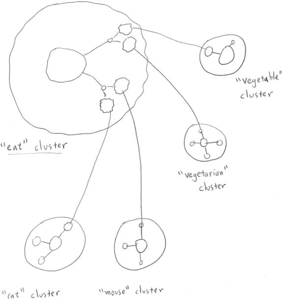
Figure 4

The expression in terms of Hebbian Logic clusters of the relationships

eat(cat, mouse) and eat(vegetarian, vegetable)

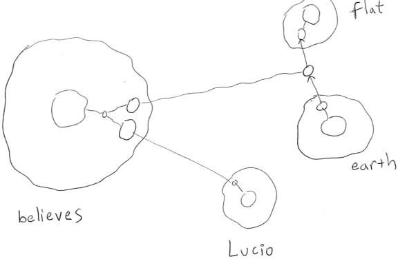
Figure 5

A Hebbian Logic representation for the relationship

believes(Lucio, earth à flat)

7.3 Variables and Quantifiers

Finally, what about variables and quantifiers? The least unnatural solution I have found so far is to introduce special neural clusters specifically identified as “variable clusters.” These must fall into two categories: ordinary variable clusters, and existential variable clusters. Two special kinds of links are then needed:

Anchor links, which form the definition of a variable cluster (for instance, to define {X so that Xàcat and Xàdog}, we create a variable cluster X and link it with anchor synapses to the “cat” and “dog” neural clusters)
Dependency links, which attach an existential variable cluster to the variable cluster on which it depends (e.g. in “For all X, there exists a Y so that …”, the variable cluster for Y has a dependency link to the variable cluster for X)

Because this is a significant addition to the basic Hebbian Logic Network framework, we use the term “Variable-Enhanced Hebbian Logic Networks” to indicate a Hebbian Logic network with these extra cluster and link types. Figures 6 and 7 depict the use of Variable-Enhanced Hebbian Logic Networks to embody some simple logical relationships.

As noted above, we are not entirely pleased with this treatment of variables and quantifiers. However, although it’s a bit inelegant, it does not appear to have any truly serious problems that would prevent its practical embodiment in AI or neurological systems. We look forward to further refinement of these ideas as the Hebbian Logic framework evolves.

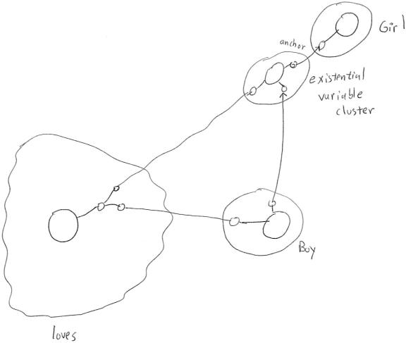
Figure 7

Representation of

“There is a girl G, so that for every boy B, B loves G”

using Variable-Enhanced Hebbian Logic

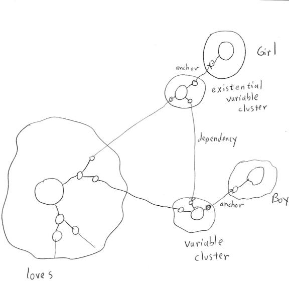
Figure 7

Representation of

“For each boy B, there exists some girl G so that B loves G”

(an example of quantifier binding in which an existential quantifier

has a Skolem-function dependency on a universal quantifier)

using Variable-Enhanced Hebbian Logic

7.4 Neural Representation of Complex Procedures

Once one can represent complex variable expressions in terms of networks neural clusters, then one can essentially represent anything. For example, there is the possibility for very subtle interrelations between declarative and procedural knowledge, of a sort that does not exist in any standard neural network architecture. This brief section contains some observations on this topic.

Declarative and procedural knowledge are different, but, much of mental activity consists of interactions between the two types of knowledge. This interaction comes in two key forms: procedures that measure relationship between facts, and procedures that are “implicitly declarative” in that they embody information about the execution of procedures. We briefly touch both of these here.

7.4.1 Procedures that Evaluate Facts

How does one define, in neural network terms, a procedure that represents a relationship between two pieces of declarative knowledge? There are two things to consider: inputs and outputs.

First, inputs. How can a neurally-implemented procedure take a neurally-implemented fact as input? Well, if each piece of declarative knowledge is represented as a subnetwork weight state, then, it is easy to have a procedure-implementing subnetwork P that controls its output based on the activation state of the subnetwork defined on its Input neurons. A procedure with multiple input arguments may be defined by interpreting the input set as multipartite, i.e. Input = Input₁ È… È Input_n .

Next, what about outputs? If we want a procedure that judges the extent of a relationship between two or more facts, then we want a procedure that outputs an uncertain truth value, i.e. a value in [0,1]. One way to do this is to consider a procedure whose “effective output” is the total activation of its Output neurons over a certain period of time. This will of course not be normalized to [0,1], but other procedures that take the output of the procedure as input can treat it as if it were normalized to [0,1], yielding the same effect implicitly.

7.4.2 Procedures that Embody Facts about Procedure Execution

Suppose a procedure is represented as a subnetwork. The fact that a procedure, over a certain period of time, takes certain inputs and produces certain outputs, is then a subnetwork activation time pattern. We may then have another procedure that outputs “true” to the extent that its input consists of this particular subnetwork activation time pattern.

8. Comments on AI and Cognitive Science

Clearly, the ideas presented here require further exploration – via at least the three avenues of mathematics, computer simulations, and biological research. Key concepts have been left semi-formal, important phenomena have been treated only by means of evocative examples, etc. But, even at this stage, it seems well worth exploring the conceptual significance of the approach, hypothetically assuming its overall validity.

What I have sought here is to show, in the abstract, how symbolic logical reasoning may emerge naturally from neural net dynamics. A bridge has been built between a (semi-local) variant of Hebbian learning, and a variant of uncertain logic. The construction of this bridge has not required any esoteric materials, simply an improvisation on the old and illustrious “cell assembly” concept, augmented by the new concept of “logic-friendliness” and a few related ideas.

It’s clear that Hebbian learning in the brain involves manifold complexities not even lightly touched by the present simplistic formalization. Our understanding of the dependence of real-brain Hebbian learning on particular neurotransmitters and their interactions is barely beginning. What has been done here is to describe a model system, qualitatively and conceptually similar to the brain but simpler, which gives rise to logic on an emergent level. It is hoped that this model system will be of some use in unraveling the deeper and subtler dynamics of real-brain Hebbian learning. For we conjecture that the essence of real-brain Hebbian learning is going to be somewhat similar to the Hebbian learning variant described here – though undoubtedly more complex.

As regards the implications of the present ideas for artificial intelligence, we consider this a largely separate issue. We have explained here how we believe neural networks can give rise to logical inference, on an emergent level. Logical inference is far from all there is to intelligence; however, our opinion is that handling logic is the hardest part of outlining a neural net based design for AI. For example, we suspect that nearly all of our (non neural net based) Novamente AI design could be mapped into a neural net architecture, defined along lines similar to those described here, using inheritance, similarity, general procedures, lists, and uncertain logical reasoning in a neural net framework. PTL is only one aspect of Novamente, but, the non-PTL Novamente are primarily much more neural-nettish already; and one major non-neural-nettish aspect of the design, evolutionary programming, has been shown in (Goertzel, 1993) to be approximable by neural net learning (in the context of a discussion of crossover between neural maps in a Neural Darwinist framework). Above we have given a few ideas along these lines, in the guise of notes on a “logic-friendly neural net architecture.”

However, the possibility of a formal neural network approach to AI does not imply the desirability of such an approach. In fact we are unsure of the value of such an enterprise – though, of course, highly curious. Clearly, a detailed simulation of the human brain in silico would have a great deal of value; but this is a very different thing from an abstracted formal neural network model of the sort described here. The critical question is: What are the AI advantages of using a Hebbian Logic representation of probabilistic inference, as opposed to a more symbolic and direct PTL representation such as is used in Novamente? It seems possible that using a cell-assembly-based knowledge representation and leaving inference on the emergent level, somehow provides more lower-level creativity than is obtained by using a semantic net representation and doing explicit inference on the nodes of the semantic net. But this is purely a speculation, and we’re not at all sure it’s accurate.

To explore this question in a serious way one needs to ask what this posited potential “creativity” really might consist of. Reasoning on existing concepts is clearly better done by explicitly logical methods. The creation of new concepts, on the other hand, is done in an interesting and different way using the attractor based representation. The question is whether this approach to concept formation is better than alternate approaches that are more natural in the semantic net approach – and, more pointedly, whether attractor based Hebbian nets somehow provide a special symmetry between reasoning and concept formation that is not present in the inferential semantic net approach. It may well be that is that using evolutionary methods for concept formation on the semantic net level (as is done in Novamente), is at least as creatively productive as concept formation that occurs because of cell assembly interaction in neural nets.

Perhaps the cognitively important thing is just that one has a flexible representation of concepts, and that it’s possible to reason about relations between concepts and to create new concepts by fusing, splitting and syntactically combining existing concepts. Different ways of carrying out these tasks will have different strengths both in terms of their ability, and in terms of their computational efficiency and simplicity. Hebbian logic and cell-assembly-based knowledge representation are particularly natural for brain hardware, whereas semantic nets with explicit inference seem to be more natural for von Neumann hardware.

If this line of thinking is correct then, in the end, the symbolic/subsymbolic distinction may well turn out to be a bit of a red herring. When one implements semantic nets in a way that’s amenable to effective use of uncertain term logic and productive concept formation, one arrives at a complex, self-organizing dynamical system that has more to do with an attractor neural net than with a typical static semantic network reasoned upon by predicate logic.

All these are big and fascinating issues, and we do not pretend to have resolved them in this paper. What we have attempted, however, is to articulate a newly explicit framework for exploring and analyzing issues at the symbolic/subsymbolic fringe. The relation between symbolic reasoning and subsymbolic dynamics lies right at the center of AI, yet there is surprisingly little work explicitly addressing this relationship in a concrete way, either experimentally or mathematically. If AI is to significantly progress, this must change, and this is the spirit in which the Hebbian Logic framework is offered.

References

Bi, G. and Poo, M. (1999). Distributed synaptic modification in neural networks induced by patterned stimulation. Nature 401, p. 792-796
Curry, Haskell and Robert Feys (1958). Combinatory Logic.
Edelman, Gerald (1988). Neural Darwinism. Basic Books.
Field and Harrison (1988). Functional Programming. Addison-Wesley.
Goertzel, Ben (1993). The Evolving Mind. Gordon and Breach.
Goertzel, Ben (1997). From Complexity to Creativity. Plenum Press.
Goertzel, Ben, Ken Silverman, Cate Hartley, Stephan Bugaj, Mike Ross (2000). The Baby Webmind Project, Proceedings of AISB 2000
Goertzel, Ben (2002). Creating Internet Intelligence. Plenum Press.
Goertzel, Ben, Izabela Freire, Jeff Pressing, Cassio Pennachin, Guilherme Lamacie (2003). Probabilistic Term Logic. Novamente LLC technical report.
Goertzel, Ben, Cassio Pennachin (2003). Novamente: Design for an Artificial General Intelligence. Novamente LLC technical report
Hebb, Donald (1948). The Organization of Behavior.
Tao, H., Li Zhang, G. Bi, M. Poo (2000). Selective presynaptic propagation of long-term potentiation in defined neural networks. J. Neuroscience 20(9), pp. 3233-43
Wang, Pei (1995). Non-Axiomatic Reasoning System. PhD Thesis, U. of Indiana at Bloomington, Department of Computer and Cognitive Sciences

[1] “Weight of evidence” is a NARS/PTL concept denoting the number of items of evidence used in estimating a probability, normalized into the interval [0,1]

[2] The author is indebted to Izabela Freire for this observation. Prior to a conversation with her on the topic, he erroneously believed that a more complex workaround was needed to deal with this problem.